Home > ANSYS HFSS 教學 > Stripline Differential Pair

 

本文始於2009年筆者初入SI、PI領域時，使用Ansoft HFSS v10.0完成操作，模擬步驟與說明較為簡略，也沒有附上範例檔。2012年重新以HFSS v14.0撰寫本文，並附上範例檔供學習參考。此例的重點在了解Driven Terminal下wave port + de-embed使用，與differential pair的odd mode、even mode field，並做特性阻抗最佳化求解。

1. Get Started

2. Create 3D Model

3. Create Wave Port Excitation

4. Analysis Setup

5. Create Reports

   -- S_DD11 plot

   -- Export S-parameter

6. Create Field Overlay

7. Design Optimize

8. Animate Field Overlay

9. Export Differential S-parameter

10. Transfer Diff. S-parameter to Single-end S-parameter

11. 問題與討論

    11.1 De-embed有什麼優點?

    11.2 在HFSS中，如何觀察Zin(從port往系統網路看)、埠端阻抗(port Zo)與傳輸線特性阻抗(Zo)?

    11.3 為何此例在HFSS內模擬時，不需要設background (air box)? 又此例stripline的reference plane在哪裡?

    11.4 什麼時候用wave port，甚麼時候用lump port?此例如果改成lump port，結果會不會相同?

    11.5 如果step3.3不用de-embed，而是真正建一段線長1000mils的傳輸線取代本例100mils線長+900mils de-embed，結果相同嗎?

12. 參考資料

1. Get Started 

1.1 Setting Tool Options

Tools \ Options \ HFSS Options： 被複製的幾何形物件，默認有一樣的邊界特性

Tools \ Options \ Modeler Options：

1.2 Open a new project：File \ New 

如果希望一開啟HFSS就已經有一個new project，請從Tools \ Options \ General Options：

1.3 Set Solution Type：HFSS \ Solution Type, choose [Driven Terminal] for this example

讀者可以用Help搜尋[Solution Type]的說明：

[Driven Mode] is for calculating the mode-based S-parameters of passive, high-frequency structures such as microstrips, waveguides, and transmission lines which are "driven" by a source, and for computing incident plane wave scattering. The S-matrix solution will be expressed in terms of the incident and reflected powers of waveguide modes.

[Driven Terminal] is for calculating the terminal-based S-parameters of passive, high-frequency structures with multi-conductor transmission line ports. This solution type results in a terminal-based description in terms of voltages and currents.

[Eigen Mode] is for calculating the Eigenmodes, or resonances, of a structure. The Eigenmode solver finds the resonant frequencies of the structure and the fields at those resonant frequencies. Eigenmode designs cannot contain design parameters that depend on frequency.

[Transient] is for calculating problems in the time domain. It employs a time-domain "transient" solver. Typically applications include (The mode appears from HFSS 13)

1.4 Set Model Units：Modeler \ Units, select "mil"

小心不要選錯成[mile]，差一字可是差很多的

1.5 Set Default Material：直接從工具列選擇

在"Search by Name"欄位內填入"pec" (means perfect conductor)，下面視窗內即會自動搜尋到該名稱的材質，然後按"確定"即可。這個設定步驟，是確保我們等等畫的signal trace材質是良導體(默認pec)。

雖然本例使用的材質介電係數是不隨頻率變化，但HFSS可設定隨頻率變化的介電係數，請參閱

2. Create 3D Model 

目標是模擬線寬W=6mils、線距S=18mils、線長1000mils的differential pair，堆疊結構則是線銅厚0.7mils，訊號線夾在高度26mils的substrate中，介電係數4.4，沒有另外再畫其他的金屬平面 。

2.1 Create trace 1, trace 2

2.1.1 畫傳輸線實體結構有兩種方法，HFSS v12以前的文件是用Drow \ Box，HFSS v13以後的文件是用Draw\Line + CreatePolyline。後者在畫傳輸線的應用上，會方便許多。

• Draw \ Box按下後，下方狀態列會出現座標輸入欄位 ，請輸入對角兩點的座標(基準座標與相對座標)

接著會彈出物件屬性編輯窗，將原本"position"該列中的9mil改寫成S/2，接著在跳出的變數定義窗中定義S=18mil；同理定義W=6mil。然後選擇"Attribute"標籤頁，更改Name type=trace1

• Draw \ Line from (0, 0, 0) to (100, 0, 0), and rename in [Attribute] tab as "trace1"

   Edit \ Select All

   Edit \ Arrange \ Move from (0, 0, 0) to (0, 9, 0), and a Properties window will launch

2.1.2 上述步驟完成後，可以從View \ Fit All \ Active View或按Ctrl+D 檢視全貌

2.1.3 先在History Tree內由Object \ pec \ trace1選定上一步驟所繪製的trace1，按滑鼠右鍵選擇"Mirror"

以上步驟，也可以由Edit \ Select All Visible + Edit \Duplicate \ Mirror完成。

此時游標變成一個較大的黑色實心菱形，以指定鏡射方向；當然也可以透過輸入基準座標與相對座標來指定鏡射方向。(往-Y軸方向翻)

接著會彈出物件屬性編輯窗，選擇"Attribute"標籤頁，更改Name type=trace2

2.2 Create Substrate of permittivity =4.4

直接從工具列選擇 ，按"Add Material"，新建一個電介係數為4.4的材質，命名為My_FR4

畫包圍傳輸線的substrate (dielectric)實體結構同樣有兩種方法

• Draw \ Box按下後，請輸入基準座標與相對座標(0,-100,-13)(100,200,26)，然後在屬性設定窗中，在"Attribute"標籤頁內，將名稱改成substrate，透明度Transparency改成0.8

• Draw \ Line from (0, 0, 0) to (100, 0, 0)，然後其Properties內的Type選[Rectangle]，Width/Diameter=200，High=26，透明度設0.

3. Create Wave Port Excitation 

3.1 Create wave port excitation p1, p2

3.1.1 Edit \ Select \ Faces
       Edit \ Select \ By Name

3.1.2 HFSS \ Excitations \ Assign \ Wave Port

將此wave port命名為p1， 然後按OK。

導體延伸到air box，wave port直接下在air box的面上，這是典型的external wave port；另有一種internal wave port的做法，需要在wave port的另一邊貼一個導體平面。

同理在對面的face也建wave port。

3.2 Set Differential Pairs

HFSS \ Excitations \ Differential Pairs 或到Project window內的Excitation點右鍵選擇[Differential Pairs]

連續按兩次[New Pair]

3.3 Set de-embed distance of the transmission line

HFSS \ List 選擇[Excitation] tab，也可以看到p1, p2

選擇p2，然後按"Properties"，[Deembed]打勾，[Deembed Distance]填-900mil

[Deembed]這是HFSS在模擬傳輸線時，一個很好用的功能；user只需建一小段的固定傳輸線模型，然後設定De-embed Distance，即可任意調整傳輸線長度，不需rerun而得到模擬結果。以此例來說，我們想要模擬1000mils長的傳輸線，但我們所建的模型只有100mils，所以設定De-embed Distance=-900mils(即延長傳輸線長度900mils)。設定後可以看到一根粗的藍色線，標示傳輸線長度的延伸。

3.4 Verify the boundary：HFSS \ Boundary Display (Solver View)

背景環境有默認的boundary

本例不需要另外框一個背景輻射空間，原因是因為訊號線已經被包在一個已經有設定屬性的材質裡了(substrate, My_FR4)，且因為wave port正好佈滿兩側，wave port的四邊所延伸的四面，其邊界條件默認是Perfect Conductor。

4. Analysis Setup 

   4.1 HFSS \ Analysis Setup \ Add Solution Setup

或是按滑鼠右鍵 

[Solution Frequency]若取整個系統設計的最大考慮頻寬，mesh會切最多，模擬時間較長，但模擬也會最準。

對於天線設計，因為我們通常只在意天線操作頻帶，所以這個值可以設天線阻抗最低的操作頻點；但對於SI設計的應用，則建議取0.5/Tr值。

[Maximum Number of Passes] is the maximum number of mesh refinement cycles for HFSS to perform. 設大於2(含)就會mesh refinement，設的越大，可容許的refine tuning次數越多，模擬時消耗的記憶體也越多(一般設10~20)， 但若mesh refinement提前達到[Maximum Delta S]條件就會停下來

[Minimum Converged Passes]設定建議從1改成2，mesh refinement的次數會多一次，但可以確保meshing切的真正足夠

Zero order、First order(default)、Second order，會分別自動對應"Lambda Refinement"為Target 0.1、0.3333、0.6667，越高階order越適合用來解結構複雜的模型，但時間也會花較多。HFSS v12以後多了[Mixed Order]，建議默認用此 檔設定，會在結構較複雜或電場變化較大的地方，自動以high order處理

[Enable Iterative Solver]：The iterative solver significantly reduces memory usage, and it can also provide a savings in the solution time for large simulations.

4.2 HFSS \ Analysis Setup \ Add Frequency Sweep

或是按滑鼠右鍵

[DC Extrapolation]只有當[Sweep Type]選擇[Interpolating]才 有，且Start Frequency設0時，[DC Extrapolation]的最小頻率才能指定

[Sweep Type] 選[Discrete]就是針對指定的頻點老實求解，費時較久但較準確， 一般5GHz內的頻寬適用。[Fast]適用於 局部窄頻段內頻率響應變化大的題目，如特性振盪的頻段(resonant frequency)，可以在指定求解的頻點小範圍內精準。[Interpolating]則適用於寬頻帶(10GHz~)且頻率響應較緩和的(smooth)題目。

4.3 HFSS \ Validation Check

      HFSS \ Analyze All

5. Create Reports 

   5.1 HFSS \ Results \ Solution Data

   查看模擬過程中花多少時間，用了多少記憶體資源

查看模擬過程中做了幾次疊代才得到收斂值

總共切多少mesh

每次跑的結果不一定相同，若電腦太遜，還有可能跑一跑就Error而跑不出結果。這些訊息可以在執行過程中real time check。

5.2 S-parameter plot 

HFSS \ Results \ Create Terminal Solution Data Report \ Rectangular Plot

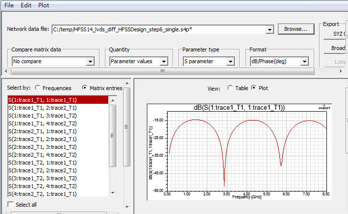
5.3 從S_DD11可以看出此1000mils的傳輸線，在2.92GHz、5.84GHz有共振點

5.4 Export S-parameter  

HFSS \ Results \ Solution Data，[Display All Freqs]打勾，按[Export Matrix Data]即可另存.snp file (.snp)

若按[Equivalent Circuit Export]，則可輸出PSpice.lib或HSPICE.sp

6. Create Field Overlay  

6.1 Set the field excitation：HFSS \ Fields \ Edit Sources，設定p1 drive，p2 terminated

或是按滑鼠右鍵

6.2 Create a field plot：HFSS \ Fields \ Fields \ E \ Mag_E (能量大小顯示)

HFSS \ Fields \ Modify Plot Attributes

或是

若從[Edit Source]修改[Phase]設定，可以看出Mag_E場圖的變化 ，下圖左是common mode，圖右是differential mode

6.3 Create a field plot：HFSS \ Fields \ Plot Fields \ E \ Vector_E (方向顯示)

HFSS \ Fields \ Modify Plot Attributes

7. Design Optimize 

在6.5<W<7.5mils，16.5<S<17.5mils求解最佳化設計

7.1 Add a parametric sweep：HFSS \ Optimetrics Analysis \ Add Parametric

7.2 Run Analysis

7.3  HFSS \ Results \ Create Terminal Solution Data Report \ Rectangular Plot

隨著線距S的增加，差分特性阻抗變大；同樣線距下，W越小特性阻抗越大。

step 7.1~7.3還不算是真的用HFSS做最佳化設計，真的最佳化求解的做法如下

7.4 Add Optimization

[HFSS] \ [Design Properties]

[HFSS] \ [Optimetrics Analysis] \ [Add Optimization]

7.5 Run Optimize Analysis

此例如果採用[Pattern Search]做最佳化，3次收斂

此例如果進採用[Quasi Newton]做最佳化，11次收斂

透過查詢on line help [Choosing an Optimizer]可知，對於少變數(2D~3D search)的簡單題目，用[Pattern Search]比用[Quasi Newton]好。但不管是[Pattern Search]或[Quasi Newton]，在做最佳化搜尋時，預設給的搜尋範圍與初始計算值，會影響最佳化搜尋的效率。

8. Animate Field Overlay 

8.1 Double click on Mag_E

8.2 Mag_E \ Animate

8.3 Setup Animation：可以分別選擇"Swept Variable"為Phase、S、W，按OK

9. Export Differential S-parameter

Follow step5.4

10. Transfer Diff. S-parameter to Single-end S-parameter

HFSS可以支持吐出single-end S-parameter as step5.4，或是differential S-parameter as step9。但如果我們並沒有3D model，只有S-parameter (.snp)，那如何在single-end與differential間做轉換呢?

Designer 6.0有提供一個非常好用的功能：Tool \ Net Data Explorer，不但可以把single-end轉differential  S-parameter，還可以把S參數轉Z參數

Edit \ Define Differential Pairs

11. 問題與討論

11.1 De-embed有什麼優點?

Ans：讀者可以把本文step3.3中的[Deembed Distance]值，改填-900mm(不需rerun)，即可看到S plot結果如下，諧振頻點從低頻到高頻(變多 變密)，S11也從-15dB下降到-24dB。透過這方式，user不需重新建模，可以快速調整結構長度，而且不需重新mesh或模擬計算。如果不用這方式，而是把3D model的長度參數設變數，那越長的結構模擬時間會增加越多。

11.2 在HFSS中，如何觀察Zin(從port往系統網路看)、埠端阻抗(port Zo)與傳輸線特性阻抗(Zo)?

Ans：在step5.2中，Category：Terminal Port Zo即是指port端阻抗，而不是傳輸線上的特性阻抗，不要搞錯了。Category：Terminal Z Parameter即是指從port往系統網路看的阻抗Z₁₁ 。而傳輸線的特性阻抗若要在HFSS查看，則要到時域裡看TDR。

11.3 為何此例在HFSS模擬時，不需要設background (air box)? 又此例stripline的reference plane在哪裡?

Ans：默認的background boundary (substrate表面)是理想導體，若不考慮reference plane的導電率，傳輸線就直接以boundary face當reference plane。為了驗證這點，我們在上下表面各貼一層Perfect E的sheet當reference plane，重新下wave port，且該wave port同時以此上下兩sheet為reference，模擬結果如下，與step5.3一模一樣

11.4 什麼時候用wave port，甚麼時候用lump port?此例如果改成lump port，結果會不會相同?

Ans：wave port是以平面能量來計算，lump port是以V/I來計算，如果lump port夠短，可以得到很接近的S-parameter模擬結果 ，除非wave port size設的不對。 一般天線或波導管設計建議用wave port，SI設計建議用lump port，但沒有絕對。Lump port也可設de-embed，也可以設成參考上下兩平面，但lump port與wave port的de-embedded是不同的。前者是K掉lump port的電感效應port calibration(所以我們建議lump port越短越好)，後者是以後處理的方式影響S參數結果，試算不同的傳輸線長度。

11.5 如果step3.3不用de-embed，而是真正建一段線長1000mils的傳輸線取代本例100mils線長+900mils de-embed，結果相同嗎?

Ans：與step5.3的模擬結果相比， 在3GHz S₁₁大約差4dB，諧振頻點約偏移3%，在6GHz S₁₁大約差12dB。故太長的wave port de-embed是會造成S₁₁誤差的 ，雖然這誤差很小，建議de-embed長度最好不要超過l/10

12. 參考資料

12.1 SI issue for high speed serial differential interconnection -- 中華大學 薛光華老師

12.2 EMC Considerations for Differential Lines , 2007

12.3 Differential Signals are NOT Immune to EMI/EMC Concerns! , 2010

12.4 HFSS v13,v12與v11的差異? -- ANSYS